# ML# Machine Learning algorithms
Supervised learning
Unsupervised learning
# Supervised learning算法通过分析这些训练样本,学习从输入到输出的映射关系,然后利用这个映射关系对新的、未见过的样本进行预测。
监督学习算法:回归 (regression)、分类 (classification)
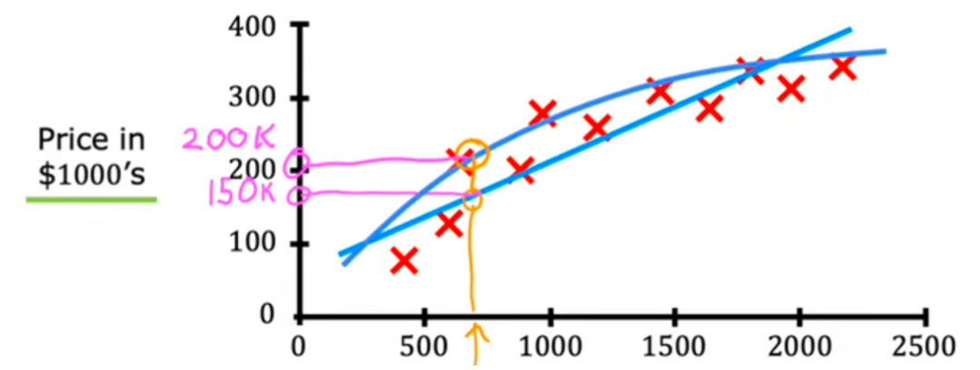
回归:从无数可能得数字中预测数字。 房价预测
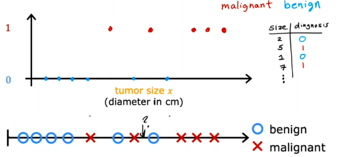
分类:只预测一小部分可能的输出 ,可能有多种输出。输入可能有多个 肿瘤诊断
# Unsupervised learning数据仅带有输入 X,没有输出标签 y,需要在数据中找到某种结构
聚类 :获取没有标签的数据并尝试自动将他们分类的集群中
比如将有相似词的文章检索放在同一组中
异常检测
降维:将大数据集压缩成一个小数据集,同时丢失尽量少的信息
# 单变量线性回归模型Notation:(符号表示法)
x $$ “input” variable
feature
$$y $$ “output” variable
“target” variable
$$m $$ number of training examples
$$(x,y) $$ single training example
$$(x^{(i)},y^{(i)}) $$ $$i^{th$$ training example
$$w$$ parameter:weight
$$b$$parameter:bias(偏差)
$$x -> f -> y(\hat{y})
\hat{y}$$可能是真实值也可能是预测值
x 是feature
f 是model,hypothesis(假设)
**单变量****线性回归****模型**$$f_{w,b}
f_{w,b}(x^{(i)})=wx^{(i)} + b$$ The result of the model evaluation at 𝑥(𝑖) parameterized by 𝑤,𝑏
python 中常用库
NumPy,一种流行的科学计算库
Matplotlib,一种用于绘制数据的常用库
1
2
3
4
5
6
7
8
9
10
11
12
13
14
15
16
17
18
19
20
21
22
23
24
25
26
27
28
29
30
31
32
33
34
35
36
37
38
39
40
41
42
43
44
45
46
47
48
49
50
51
52
53
54
55
56
57
58
59
60
61
62
63
64
import numpy as npimport matplotlib.pyplot as pltplt.style.use('./deeplearning.mplstyle' ) x_train = np.array([1.0 , 2.0 ]) y_train = np.array([300.0 , 500.0 ]) print (f"x_train = {x_train} " )print (f"y_train = {y_train} " )print (f"x_train.shape: {x_train.shape} " )m = x_train.shape[0 ] print (f"Number of training examples is: {m} " )i = 0 x_i = x_train[i] y_i = y_train[i] print (f"(x^({i} ), y^({i} )) = ({x_i} , {y_i} )" )plt.scatter(x_train, y_train, marker='x' , c='r' ) plt.title("Housing Prices" ) plt.ylabel('Price (in 1000s of dollars)' ) plt.xlabel('Size (1000 sqft)' ) plt.show() def compute_model_output (x, w, b ): """ Computes the prediction of a linear model Args: x (ndarray (m,)): Data, m examples w,b (scalar) : model parameters Returns f_wb (ndarray (m,)): model prediction """ m = x.shape[0 ] f_wb = np.zeros(m) for i in range (m): f_wb[i] = w * x[i] + b return f_wb tmp_f_wb = compute_model_output(x_train, w, b,) plt.plot(x_train, tmp_f_wb, c='b' ,label='Our Prediction' ) plt.scatter(x_train, y_train, marker='x' , c='r' ,label='Actual Values' ) plt.title("Housing Prices" ) plt.ylabel('Price (in 1000s of dollars)' ) plt.xlabel('Size (1000 sqft)' ) plt.legend() plt.show()
### 单变量线性回归模型 的 Cost function -- 损失函数
损失函数用于衡量预测房屋的目标价格的指标
$$J_{(w,b)} = \frac{1}{2m}\sum_{i = 1}^{m}(\hat{y}_{i}-y_{i})^2$$ => 平方误差损失函数,$$(\hat{y}-y)^2$$代表预测值和目标值之间的平方差,求和会把多个误差值累计,$$\frac{1}{m}$$代表求平均值,$$\times{2}$$为了后续求导方便
$$J_{(w,b)} = \frac{1}{2m}\sum_{i = 1}^{m}(f_{w,b}(x^{(i)})-y^{(i)})^2$$,其中 $$f_{w,b}(x^{(i)})=wx^{(i)} + b$$。
> 𝑓𝑤,𝑏(𝑥(𝑖)) 是我们的预测,即$$\hat{y}$$,例如 𝑖 使用 parameters 𝑤,𝑏
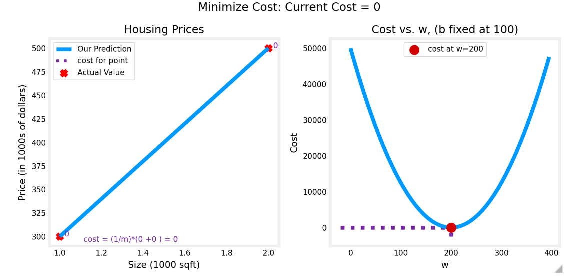
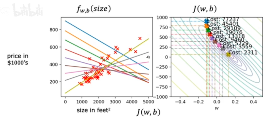
固定b的值,假设此处b=100,fw,b和Jw,b 如图所示。求w的过程就是找cost最小的过程。即minj(w,b)
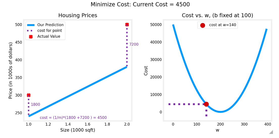
此时损失函数是一个二次函数,最低点即为cost最小的点,此时w=200,此时cost=0
> 证明: 为什么对于 $$y=wx+100$$时,其损失函数为二次函数
>
> $$J_{(w)} = \frac{1}{2m}\sum_{i = 1}^{m}(f_{w}(x^{(i)})-y^{(i)})^2
=> $$J_{(w,b)}=\frac{1}{2m}[(wx_1+100-y_1)2+(wx_2+100-y_2) 2]$$
带入 (1,300) (2,500)
= 1 2 m [ ( w − 200 ) 2 + ( 2 w − 400 ) 2 ] =\frac{1}{2m}[(w-200)^2+(2w-400)^2]
= 2 m 1 [ ( w − 2 0 0 ) 2 + ( 2 w − 4 0 0 ) 2 ]
= 1 2 m ( 5 w 2 − 2000 w + 200000 ) =\frac{1}{2m}(5w^2-2000w+200000)
= 2 m 1 ( 5 w 2 − 2 0 0 0 w + 2 0 0 0 0 0 )
general case:w,b 都是未知量
minimize J(_{w,b})$$ 求minimize后的图形如下,求最小值的一类方案是找等高线。

> 证明方式同理,展开带入得到w和b的方程,对于$$w^2+b^2$$这类图形,在三维图中为上图
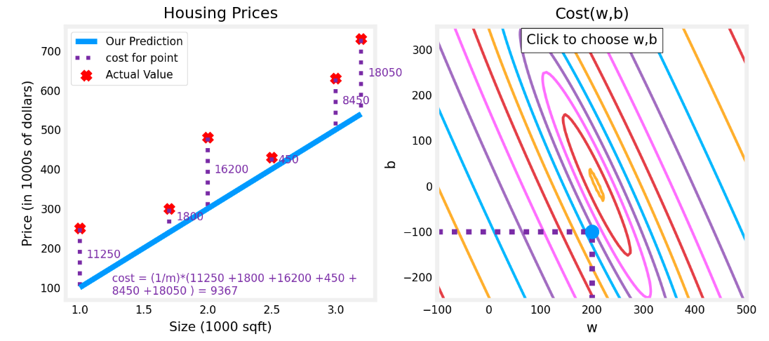
平方误差损失函数确保了“误差面”像汤碗一样凸出。它始终具有一个最小值,不像单参数一样可以直观找最低点,此时需要通过**梯度下降**找到使cost最小的点
### 梯度下降
梯度下降目标:找到使损失函数最小的w和b 即 $$min J(w1,w2,wn,b)
gradient descent algorithm 梯度下降
derivative 导数 符号 $$\alpha$$
gradient descent algorithm
repeat {
w = w - \alpha\frac{\partial J(w,b)}{\partial w} \\ b = b - \alpha\frac{\partial J(w,b)}{\partial b}$$ }, $$\alpha$$称为learning rate,(0,1),控制下降大小,偏导数控制下降方向。其中的等号为赋值运算符
梯度定义为:$$\frac{\partial J(w,b)}{\partial w} = \frac{1}{m} \sum\limits_{i = 0}^{m-1} (f_{w,b}(x^{(i)}) - y^{(i)})x^{(i)} \\ \frac{\partial J(w,b)}{\partial b} = \frac{1}{m} \sum\limits_{i = 0}^{m-1} (f_{w,b}(x^{(i)}) - y^{(i)})
包含偏导数的 python 变量的命名遵循此模式,$$\frac {\partial J (w,b)}{\partial w} $$ 记为 dj_db
方便理解,这里引入偏导数几何含义
以二元函数 $$z = f (x, y)$$ 为例,偏导数在几何中的含义如下:
f_x(x_0,y_0)$$的几何意义:固定$$y = y_0$$,此时$$z = f(x, y_0)$$可看作是关于x的一元函数。在空间直角坐标系中,$$y = y_0$$表示一个平行于xOz平面的平面,该平面与曲面$$z = f(x, y)$$相交得到一条曲线。那么偏导数$$f_x(x_0,y_0)$$就表示这条曲线在点$$(x_0,y_0,f(x_0,y_0))$$处 ,**相对于x轴方向的切线斜率** 。
梯度指向远离最小值
同时更新 w 和 b,使得取到极小值
1
2
3
4
tmp_w = w - aJ(w,b) tmp_b = b - aJ(w,b) w = tmp_w b = tmp_b
\alpha$$太小的情况,梯度下降的会很慢
$$\alpha$$过大,可能导致J(w)更大,不会达到最小值
已经在局部最小值时,梯度下降不会改变w
临近局部最小值时,导数会变得更小,每次梯度下降的程度会变的更小

### 线性回归中梯度下降
$$w = w - \alpha\frac{1}{m}\sum_{i = 1}^{m}(f_{w,b}(x^{(i)}) - y^{(i)})x^{(i)} \\ b = b - \alpha\frac{1}{m}\sum_{i = 1}^{m}(f_{w,b}(x^{(i)}) - y^{(i)})$$,其中$$f_{w,b}(x^{(i)})=wx^{(i)} + b$$,在每一步同时更新$$w,b
w = w − α 1 m ∑ i = 1 m ( f w , b ( x ( i ) ) − y ( i ) ) x ( i ) w = w - \alpha\frac{1}{m}\sum_{i = 1}^{m}(f_{w,b}(x^{(i)}) - y^{(i)})x^{(i)}
w = w − α m 1 i = 1 ∑ m ( f w , b ( x ( i ) ) − y ( i ) ) x ( i )
b = b − α 1 m ∑ i = 1 m ( f w , b ( x ( i ) ) − y ( i ) ) b = b - \alpha\frac{1}{m}\sum_{i = 1}^{m}(f_{w,b}(x^{(i)}) - y^{(i)})
b = b − α m 1 i = 1 ∑ m ( f w , b ( x ( i ) ) − y ( i ) )
f w , b ( x ( i ) ) = w x ( i ) + b f_{w,b}(x^{(i)})=wx^{(i)} + b
f w , b ( x ( i ) ) = w x ( i ) + b
此时损失函数只可能有全局最小值,不会有任何局部最小值
成本开始时很大,然后迅速下降。偏导数 dj_dw , dj_db 和 也变小,起初速度很快,然后变慢。如图表所示,当过程接近 “碗底” 时,由于该点的导数值较小,因此进度较慢。
上图是利用类等高线法绘制的图,即和 J (w,b) 平面的切线
# 多类特征
x_1,x_2,x_3...x_j$$ 表示第j个feature
n 表示 number of feature
$$\vec{x}^{(i)}$$第i个训练数据集,
$$x_j^{(i)}$$value of feature j in i training example

$$f_{w,b}(x)=w_1x_1+w_2x_2+...+w_nx_n+b
w ⃗ = [ w 1 w 2 w 3 . . . w n ] \vec{w}=[w_1 w_2 w_3 ... w_n]
w = [ w 1 w 2 w 3 . . . w n ]
x ⃗ = [ x 1 x 2 x 3 . . . x n ] \vec{x}=[x_1 x_2 x_3 ... x_n]
x = [ x 1 x 2 x 3 . . . x n ]
b is a number
==> $$f_{\vec {w},b}(\vec {x})=\vec {w}\cdot\vec {x}+b$$ ==》 多元线性回归 (multiple linear regression) np.dot (w,x)+b
f w ⃗ , b ( x ⃗ ) = ∑ i = 1 n ( w j x j ) + b f_{\vec{w},b}(\vec{x})=\sum_{i = 1}^{n}(w_jx_j)+b
f w , b ( x ) = i = 1 ∑ n ( w j x j ) + b
# 多变量损失函数
J(\mathbf{w},b) = \frac{1}{2m} \sum\limits_{i = 0}^{m-1} (f_{\mathbf{w},b}(\mathbf{x}^{(i)}) - y^{(i)})^2$$,$$这里 f_{w,b}({x^{(i)}})=w\cdot x^{(i)}+b$$,$$w,x^{(i)}$$是向量
### 多元线性回归梯度下降
$$w_j=w_j - \alpha\frac{\partial J(\vec{w},b)}{\partial w_j} \\ b=b - \alpha\frac{\partial J(\vec{w},b)}{\partial b}
w_n = w_n - \alpha\frac{1}{m}\sum_{i = 1}^{m}(f_{\vec{w},b}(\vec{x}^{(i)}) - y^{(i)})x_n^{(i)} \\ b = b - \alpha\frac{1}{m}\sum_{i = 1}^{m}(f_{\vec{w},b}(\vec{x}^{(i)}) - y^{(i)}) $$Simultaneously update wj (for j=1...n) and b
normal equation 一种只适用于线性回归求解w,b的方案,这种方案不需要迭代。但是feature特别大时候计算很慢
### 特征缩放
对于范围太大的xj,会使梯度下降的慢
缩放后使特征的取值范围相似
实质上是将每个正特征除以其最大值,或者更一般地说,使用 (x-min)/(max-min) 按其最小值和最大值对每个特征进行重新缩放。两种方法都将特征归一化到 -1 和 1 的范围,其中前一种方法适用于简单的正特征,而后一种方法适用于任何特征。

特征缩放的方式1:mean normalization(归一化)
$$\mu$$是均值,$$\mu_j = \frac{1}{m} \sum_{i=0}^{m-1} x^{(i)}_j
x 1 = x 1 − μ m a x − m i n x_1= \frac{x_1-\mu}{max-min}
x 1 = m a x − m i n x 1 − μ
特征缩放的方式 2:Z-score normalization
\sigma$$ 标准差,$$\sigma^2_j = \frac{1}{m} \sum_{i=0}^{m-1} (x^{(i)}_j - \mu_j)^2$$,在 z 得分归一化后,所有要素的平均值均为 0,标准差为 1。
$$x_1= \frac{x_1-\mu_1}{\sigma_1}$$ ==》 $$x_j^{(i)}= \frac{x_j^{(i)}-\mu_j}{\sigma_j}
特征缩放目标:对于每个 xj,缩放到 $$-1<=x_j <=1$$
当然比如 - 3,3 也是可以接受的
# 成本等值线查看特征缩放的另一种方法是根据成本等值线查看。当特征尺度不匹配时,等值线图中的成本与参数图是不对称的。
在下图中,参数的尺度是匹配的。左图是 w [0] 的成本等值线图,即平方英尺与 w [1],归一化特征之前的卧室数量。该图非常不对称,完成等值线的曲线不可见。相反,当特征被规范化时,成本等值线要对称得多。结果是,在梯度下降期间对参数的更新可以使每个参数的进度相同。
convergence 收敛
# 判断梯度下降是否收敛
或者通过 J (w,b) 减少量小于等于 $$\epsilon$$
尝试先用很小的学习率,如果损失函数随着迭代次数变多而变大,那么可能代码存在问题
比如 0.001 -> 0.003 -> 0.01 -> 0.03 -> 0.1
# 特征工程梯度下降是通过强调其相关参数来为我们选择 “正确” 的特征
较小的权重值意味着不太重要 / 正确的特征,在极端情况下,当权重变为零或非常接近零时,关联的特征在将模型拟合到数据时没有用。
# 多项式回归 polynomial regressionf w ⃗ , b ( x ) = w 1 x + w 2 x 2 + w 3 x 3 + b f_{\vec{w},b}(x)=w_1x+w_2x^2+w_3x^3+b
f w , b ( x ) = w 1 x + w 2 x 2 + w 3 x 3 + b
f w ⃗ , b ( x ) = w 1 x + w 2 x 0.5 + b f_{\vec{w},b}(x)=w_1x+w_2x^{0.5}+b
f w , b ( x ) = w 1 x + w 2 x 0 . 5 + b
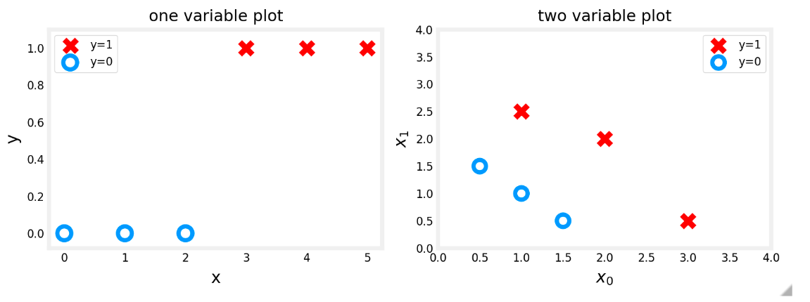
# 分类分类问题的示例包括:将电子邮件识别为垃圾邮件或非垃圾邮件,或确定肿瘤是恶性还是良性。特别是,这些是二元 分类的示例,其中有两种可能的结果。结果可以用 “积极”/ “消极 ” 成对来描述,例如 “是”/“否”、“真”/“假” 或 “1”/“0”。
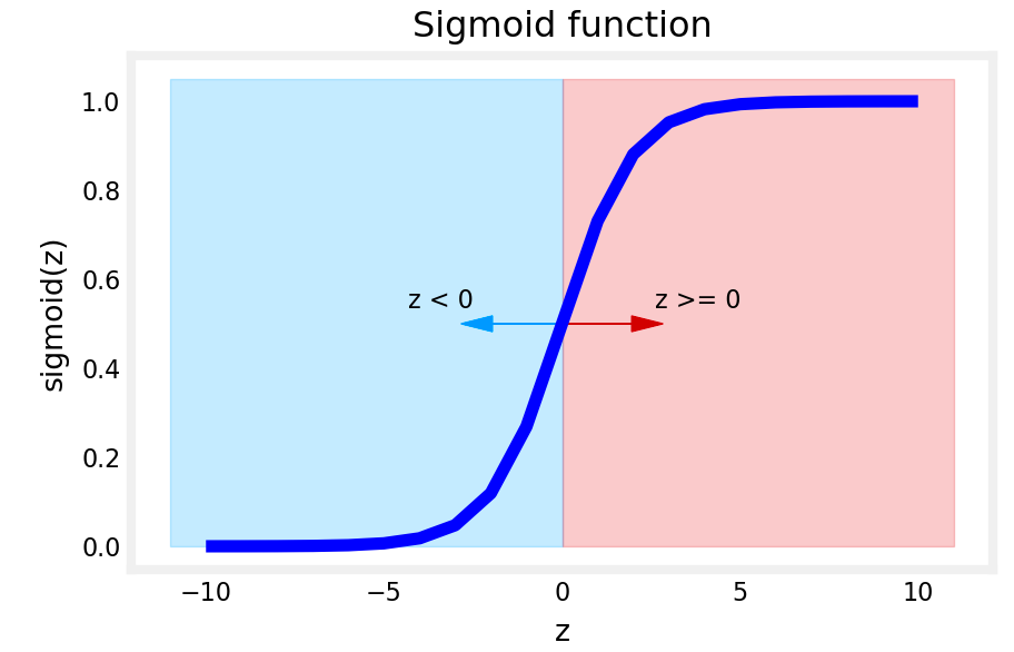
# 逻辑回归# sigmoid Function – 一种激活函数通过使用 “sigmoid 函数” 来实现,该函数将所有输入值映射到 0 到 1 之间的值。
g(z)= \frac{1}{1+e^{-z}}$$,$$0
1
2
3
4
5
6
7
8
9
10
11
12
13
14
15
16
17
18
19
20
21
def sigmoid (z ): """ Compute the sigmoid of z Args: z (ndarray): A scalar, numpy array of any size. Returns: g (ndarray): sigmoid(z), with the same shape as z """ g = 1 /(1 +np.exp(-z)) return g z_tmp = np.arange(-10 ,11 ) y = sigmoid(z_tmp) np.set_printoptions(precision=3 ) print ("Input (z), Output (sigmoid(z))" )print (np.c_[z_tmp, y])
#### Logistic Regression
$$z=\vec{w}\cdot\vec{x}+b
==> $$f_\vec{w},b}(\vec{x})=g(\vec{w}\cdot\vec{x}+b)=\frac{1}{1+e【 {-(\vec{w 】 \cdot\vec{x}+b)}}=P(y=1|x;\vec{w},b)$$
# Decision boundaryz = 0
要从 Logistic 回归模型获得最终预测 ( 𝑦=0y=0 或 𝑦=1y=1 ),我们可以使用以下启发式 -
如果 𝑓𝐰,𝑏(𝑥)>=0.5 , 预测 𝑦=1
如果 𝑓𝐰,𝑏(𝑥)<0.5 , 预测 𝑦=0
1
2
3
4
5
6
7
8
9
10
11
# Plot sigmoid(z) over a range of values from -10 to 10 z = np.arange(-10 ,11 ) fig,ax = plt.subplots(1 ,1 ,figsize= (5 ,3 )) # Plot z vs sigmoid(z) ax.plot(z, sigmoid(z), c= "b") ax.set_title("Sigmoid function") ax.set_ylabel('sigmoid(z)' ) ax.set_xlabel('z' ) draw_vthresh(ax,0 )
阴影区域(线下)中的任何点都分类为 𝑦=0。线上或上方的任何点都归类为 𝑦=1 。这条线被称为 “决策边界”。
# Logistic 损失函数i=1…m training example
j=1…n feature
traget y
逻辑回归的平方误差
J(w,b) = \frac{1}{2m} \sum\limits_{i = 0}^{m-1} (f_{w,b}(x^{(i)}) - y^{(i)})^2$$, $$f_{w,b}(x^{(i)}) = sigmoid(wx^{(i)} + b )
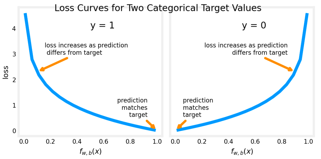
逻辑回归损失函数
此处 L (f) == loss (f)
J ( w ⃗ , b ) = 1 m ∑ i = 1 m L ( f w ⃗ , b ( x ⃗ ( i ) ) − y ( i ) ) J(\vec{w},b) = \frac{1}{m}\sum_{i = 1}^{m}L(f_{\vec{w},b}(\vec{x}^{(i)}) - y^{(i)})\\
J ( w , b ) = m 1 i = 1 ∑ m L ( f w , b ( x ( i ) ) − y ( i ) )
L(f_{\vec{w},b}(\vec{x}^{(i)}),y^{(i)}) = \begin{cases} -\log(f_{\vec{w},b}(\vec{x}^{(i)})) & \text{if } y^{(i)} = 1 \\ -\log(1 - f_{\vec{w},b}(\vec{x}^{(i)})) & \text{if } y^{(i)} = 0 \end{cases}$$,$$f_{w,b}(x^{(i)})=g(w\cdot x^{(i)}+b)$$,g是sigmoid函数
可以把上式结合一个公式,此处y(i)=0或1 $$L(f_{\vec{w},b}(\vec{x}^{(i)}) - y^{(i)})=-y^{(i)}\log\left(f_{\vec{w},b}(\vec{x}^{(i)})\right)-(1 - y^{(i)})\log\left(1 - f_{\vec{w},b}(\vec{x}^{(i)})\right)
1
2
3
4
5
6
7
8
9
10
11
12
13
14
15
16
17
18
19
20
21
22
23
def compute_cost_logistic (X, y, w, b ): """ Computes cost Args: X (ndarray (m,n)): Data, m examples with n features y (ndarray (m,)) : target values w (ndarray (n,)) : model parameters b (scalar) : model parameter Returns: cost (scalar): cost """ m = X.shape[0 ] cost = 0.0 for i in range (m): z_i = np.dot(X[i],w) + b f_wb_i = sigmoid(z_i) cost += -y[i]*np.log(f_wb_i) - (1 -y[i])*np.log(1 -f_wb_i) cost = cost / m return cost
# 逻辑回归梯度下降repeat {
w_j = w_j - \alpha\left[\frac{1}{m}\sum_{i = 1}^{m}(f_{\vec{w},b}(\vec{x}^{(i)}) - y^{(i)})x_j^{(i)}\right] \\ b = b - \alpha\left[\frac{1}{m}\sum_{i = 1}^{m}(f_{\vec{w},b}(\vec{x}^{(i)}) - y^{(i)})\right]$$,$$f_{\vec{w},b}(\vec{x})=\frac{1}{1+e^{-(\vec{w}\cdot\vec{x}+b)}}$$ }, simultaneous updates on 𝑤𝑗 for all j
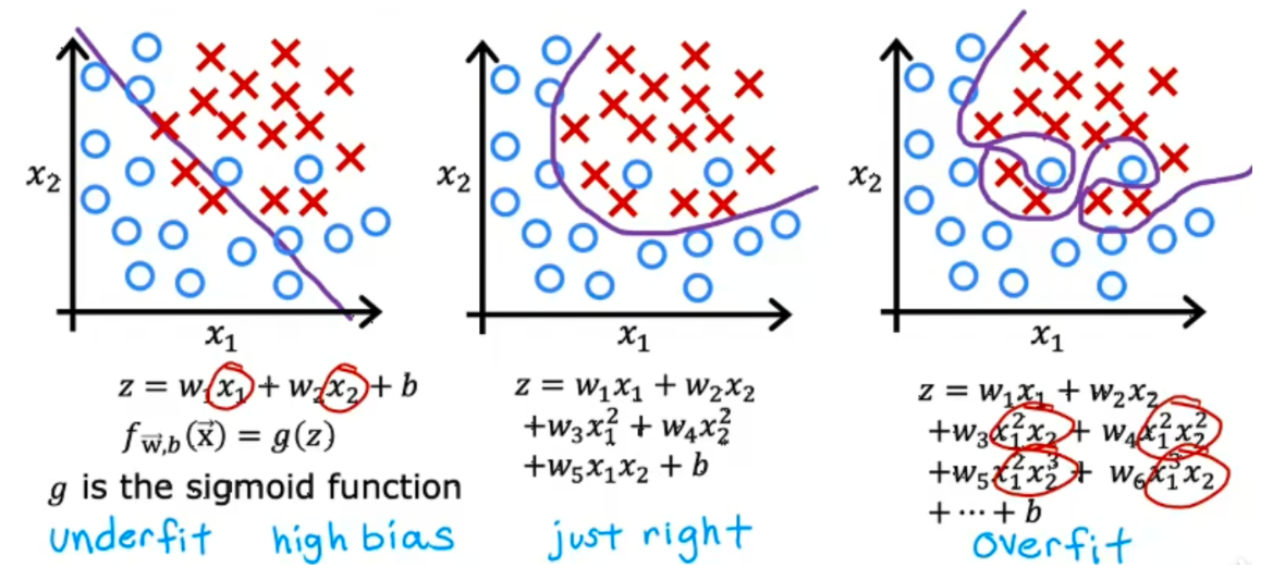
### 过拟合
regression
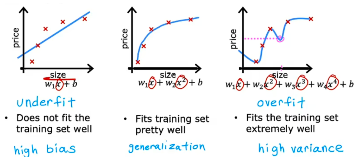
图一欠拟合(underfitting),高偏差(high bias)
图二中泛化更好,可以预测没有出现过的数据
图三过拟合(overfitting),可以称为有高方差(high variance)
classification
解决过拟合:
获取更多数据可以解决过拟合
使用更少的特征也可以解决过拟合
正则化:保留所有特征,减少参数大小,解决特征过大
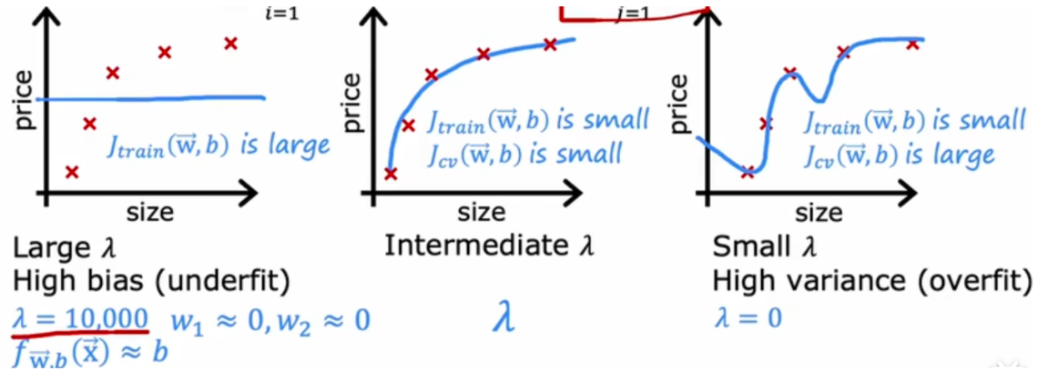
### 正则化
#### 成本函数正则化线性回归的方程
$$J(\vec{w},b)=\frac{1}{2m}\sum_{i = 1}^{m}(f_{\vec{w},b}(\vec{x}^{(i)}-\vec{y}^{(i)})^2+\frac{\lambda}{2m}\sum_{j = 1}^{n}w_j^2$$,$$\frac{1}{2m}\sum_{i = 1}^{m}(f_{\vec{w},b}(\vec{x}^{(i)}-\vec{y}^{(i)})^2$$是mean squared error ,$$\frac{\lambda}{2m}\sum_{j = 1}^{n}w_j^2$$ regularization term,$$f_{\mathbf{w},b}(\mathbf{x}^{(i)}) = \mathbf{w} \cdot \mathbf{x}^{(i)} + b
m i n w ⃗ , b J ( w ⃗ , b ) = m i n w ⃗ , b [ 1 2 m ∑ i = 1 m ( f w ⃗ , b ( x ⃗ ( i ) − y ⃗ ( i ) ) 2 + λ 2 m ∑ j = 1 n w j 2 ] min _{\vec{w},b}J(\vec{w},b)=min _{\vec{w},b}[\frac{1}{2m}\sum_{i = 1}^{m}(f_{\vec{w},b}(\vec{x}^{(i)}-\vec{y}^{(i)})^2+\frac{\lambda}{2m}\sum_{j = 1}^{n}w_j^2]
m i n w , b J ( w , b ) = m i n w , b [ 2 m 1 i = 1 ∑ m ( f w , b ( x ( i ) − y ( i ) ) 2 + 2 m λ j = 1 ∑ n w j 2 ]
\lambda$$过大,会导致欠拟合,过小会导致过拟合
1
2
3
4
5
6
7
8
9
10
11
12
13
14
15
16
17
18
19
20
21
22
23
24
25
26
27
28
def compute_cost_linear_reg (X, y, w, b, lambda_ = 1 ): """ Computes the cost over all examples Args: X (ndarray (m,n): Data, m examples with n features y (ndarray (m,)): target values w (ndarray (n,)): model parameters b (scalar) : model parameter lambda_ (scalar): Controls amount of regularization Returns: total_cost (scalar): cost """ m = X.shape[0 ] n = len (w) cost = 0. for i in range (m): f_wb_i = np.dot(X[i], w) + b cost = cost + (f_wb_i - y[i])**2 cost = cost / (2 * m) reg_cost = 0 for j in range (n): reg_cost += (w[j]**2 ) reg_cost = (lambda_/(2 *m)) * reg_cost total_cost = cost + reg_cost return total_cost
#### 正则化线性回归梯度下降
$$ w_j = w_j - \alpha\left[\frac{1}{m}\sum_{i = 1}^{m}\left[\left(f_{\vec{w},b}(\vec{x}^{(i)}) - y^{(i)}\right)x_j^{(i)}\right] + \frac{\lambda}{m}w_j\right] \\ b = b - \alpha\frac{1}{m}\sum_{i = 1}^{m}\left(f_{\vec{w},b}(\vec{x}^{(i)}) - y^{(i)}\right)
# 正则化 logistic regression
J(\vec{w},b)=-\frac{1}{m}\sum_{i = 1}^{m}\left[y^{(i)}\log\left(f_{\vec{w},b}(\vec{x}^{(i)})\right)+(1 - y^{(i)})\log\left(1 - f_{\vec{w},b}(\vec{x}^{(i)})\right)\right]+\frac{\lambda}{2m}\sum_{j = 1}^{n}w_j^2 $$,$$f_{\mathbf{w},b}(\mathbf{x}^{(i)}) = sigmoid(\mathbf{w} \cdot \mathbf{x}^{(i)} + b)
1
2
3
4
5
6
7
8
9
10
11
12
13
14
15
16
17
18
19
20
21
22
23
24
25
26
27
28
29
30
def compute_cost_logistic_reg (X, y, w, b, lambda_ = 1 ): """ Computes the cost over all examples Args: Args: X (ndarray (m,n): Data, m examples with n features y (ndarray (m,)): target values w (ndarray (n,)): model parameters b (scalar) : model parameter lambda_ (scalar): Controls amount of regularization Returns: total_cost (scalar): cost """ m,n = X.shape cost = 0. for i in range (m): z_i = np.dot(X[i], w) + b f_wb_i = sigmoid(z_i) cost += -y[i]*np.log(f_wb_i) - (1 -y[i])*np.log(1 -f_wb_i) cost = cost/m reg_cost = 0 for j in range (n): reg_cost += (w[j]**2 ) reg_cost = (lambda_/(2 *m)) * reg_cost total_cost = cost + reg_cost return total_cost
# 正则化梯度下降repeat {
w_j = w_j - \alpha\left[\frac{1}{m}\sum_{i = 1}^{m}\left[\left(f_{\vec{w},b}(\vec{x}^{(i)}) - y^{(i)}\right)x_j^{(i)}\right] + \frac{\lambda}{m}w_j\right] \\ b = b - \alpha\frac{1}{m}\sum_{i = 1}^{m}\left(f_{\vec{w},b}(\vec{x}^{(i)}) - y^{(i)}\right)$$,$$f_{\vec{w},b} $$$$x = \begin{cases} f_{\mathbf{w},b}(x) = \mathbf{w} \cdot \mathbf{x} + b ,线性回归模型 \\ z = \mathbf{w} \cdot \mathbf{x} + b,f_{\mathbf{w},b}(x) = g(z),g(z) = \frac{1}{1+e^{-z}},Logistic回归 \end{cases}$$ }
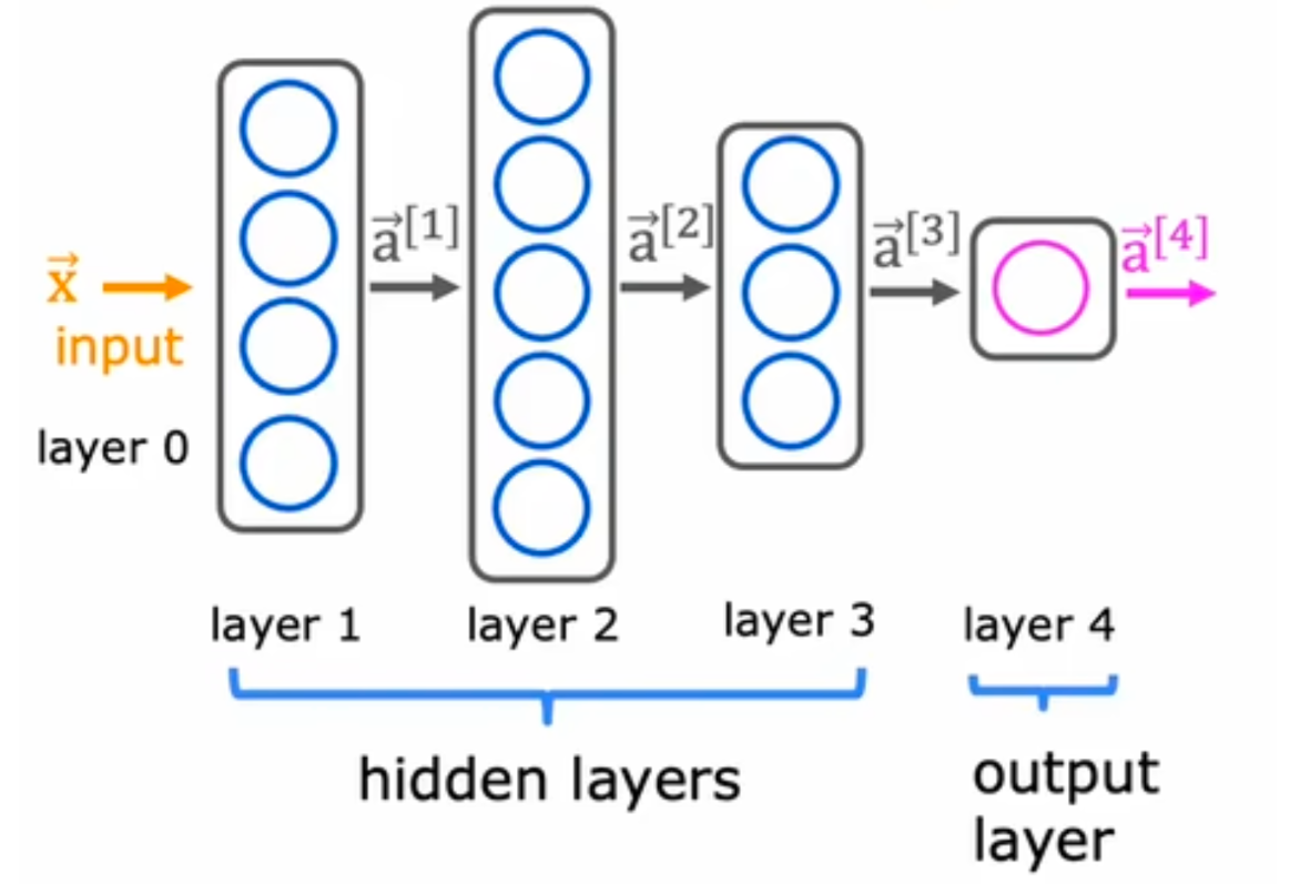
### 神经网络
input layer -> hidden layer -> output layer
$$[1] $$第一层隐藏层的输出
$$\vec{a}^{[i]}$$ i=1代表第二层隐藏层的输入
四层神经网络,一般不包含输入层
$$a_2^{[3]} = g(\vec{w}_2^{[3]} \cdot \vec{a}^{[2]} + b_2^{[3]})
a j [ l ] = g ( w ⃗ j [ l ] ⋅ a ⃗ [ l − 1 ] + b j [ l ] ) a_j^{[l]} = g(\vec{w}_j^{[l]} \cdot \vec{a}^{[l-1]} + b_j^{[l]})
a j [ l ] = g ( w j [ l ] ⋅ a [ l − 1 ] + b j [ l ] )
g 激活函数
前向传播, a [0] 到输出 a [4] ,并且随着接近输入层,隐藏单元数量变少
# TensorFlowTensorflow 是由 Google 开发的机器学习包。2019 年,Google 将 Keras 集成到 Tensorflow 中,并发布了 Tensorflow 2.0。Keras 是由 François Chollet 独立开发的框架,用于创建一个简单的、以层为中心的 Tensorflow 接口。
# 神经元与神经层1 2 3 4 5 6 7 8 9 10 11 12 13 14 15 16 17 18 19 20 21 22 23 24 25 26 27 28 29 30 31 32 33 34 35 36 37 38 39 40 41 42 43 44 45 46 47 48 49 50 51 52 53 54 55 56 57 58 59 60 61 62 63 64 65 66 67 68 69 70 71 72 73 74 75 76 77 78 79 80 81 82 83 84 85 86 87 88 89 90 91 92 93 94 95 96 97 98 99 100 101 102 103 104 105 106 107 108 109 110 111 112 113 114 115 116 117 118 119 120 121 122 123 124 125 126 127 128 129 130 131 132 133 134 135 136 137 138 139 140 141 142 143 144 145 146 147 148 149 150 151 152 153 154 155 156 157 import numpy as npimport matplotlib.pyplot as pltimport tensorflow as tffrom tensorflow.keras.layers import Dense, Inputfrom tensorflow.keras import Sequentialfrom tensorflow.keras.losses import MeanSquaredError, BinaryCrossentropyfrom tensorflow.keras.activations import sigmoidfrom lab_utils_common import dlcfrom lab_neurons_utils import plt_prob_1d, sigmoidnp, plt_linear, plt_logisticplt.style.use('./deeplearning.mplstyle' ) import logginglogging.getLogger("tensorflow" ).setLevel(logging.ERROR) tf.autograph.set_verbosity(0 ) X_train = np.array([[1.0 ], [2.0 ]], dtype=np.float32) Y_train = np.array([[300.0 ], [500.0 ]], dtype=np.float32) fig, ax = plt.subplots(1 ,1 ) ax.scatter(X_train, Y_train, marker='x' , c='r' , label="Data Points" ) ax.legend( fontsize='xx-large' ) ax.set_ylabel('Price (in 1000s of dollars)' , fontsize='xx-large' ) ax.set_xlabel('Size (1000 sqft)' , fontsize='xx-large' ) linear_layer = tf.keras.layers.Dense(units=1 , activation = 'linear' , ) linear_layer.get_weights() a1 = linear_layer(X_train[0 ].reshape(1 ,1 )) print (a1)w, b= linear_layer.get_weights() print (f"w = {w} , b={b} " )set_w = np.array([[200 ]]) set_b = np.array([100 ]) linear_layer.set_weights([set_w, set_b]) print (linear_layer.get_weights())a1 = linear_layer(X_train[0 ].reshape(1 ,1 )) print (a1)alin = np.dot(set_w,X_train[0 ].reshape(1 ,1 )) + set_b print (alin)prediction_tf = linear_layer(X_train) prediction_np = np.dot( X_train, set_w) + set_b plt_linear(X_train, Y_train, prediction_tf, prediction_np) X_train = np.array([[1.0 ], [2.0 ]], dtype=np.float32) Y_train = np.array([[300.0 ], [500.0 ]], dtype=np.float32) model = Sequential( [ tf.keras.layers.Dense(1 , input_dim=1 , activation = 'sigmoid' , name='L1' ) ] ) model.summary() logistic_layer = model.get_layer('L1' ) w,b = logistic_layer.get_weights() print (w,b)print (w.shape,b.shape)set_w = np.array([[2 ]]) set_b = np.array([-4.5 ]) logistic_layer.set_weights([set_w, set_b]) print (logistic_layer.get_weights())a1 = model.predict(X_train[0 ].reshape(1 ,1 )) print (a1)alog = sigmoidnp(np.dot(set_w,X_train[0 ].reshape(1 ,1 )) + set_b) print (alog)import numpy as npimport matplotlib.pyplot as pltplt.style.use('./deeplearning.mplstyle' ) import tensorflow as tffrom tensorflow.keras.models import Sequentialfrom tensorflow.keras.layers import Densefrom lab_utils_common import dlcfrom lab_coffee_utils import load_coffee_data, plt_roast, plt_prob, plt_layer, plt_network, plt_output_unitimport logginglogging.getLogger("tensorflow" ).setLevel(logging.ERROR) tf.autograph.set_verbosity(0 ) X,Y = load_coffee_data(); print (X.shape, Y.shape)print (f"Temperature Max, Min pre normalization: {np.max (X[:,0 ]):0.2 f} , {np.min (X[:,0 ]):0.2 f} " )print (f"Duration Max, Min pre normalization: {np.max (X[:,1 ]):0.2 f} , {np.min (X[:,1 ]):0.2 f} " )norm_l = tf.keras.layers.Normalization(axis=-1 ) norm_l.adapt(X) Xn = norm_l(X) print (f"Temperature Max, Min post normalization: {np.max (Xn[:,0 ]):0.2 f} , {np.min (Xn[:,0 ]):0.2 f} " )print (f"Duration Max, Min post normalization: {np.max (Xn[:,1 ]):0.2 f} , {np.min (Xn[:,1 ]):0.2 f} " )Xt = np.tile(Xn,(1000 ,1 )) Yt= np.tile(Y,(1000 ,1 )) print (Xt.shape, Yt.shape) tf.random.set_seed(1234 ) model = Sequential( [ tf.keras.Input(shape=(2 ,)), Dense(3 , activation='sigmoid' , name = 'layer1' ), Dense(1 , activation='sigmoid' , name = 'layer2' ) ] ) model.summary() W1, b1 = model.get_layer("layer1" ).get_weights() W2, b2 = model.get_layer("layer2" ).get_weights() print (f"W1{W1.shape} :\n" , W1, f"\nb1{b1.shape} :" , b1)print (f"W2{W2.shape} :\n" , W2, f"\nb2{b2.shape} :" , b2)model.compile ( loss = tf.keras.losses.BinaryCrossentropy(), optimizer = tf.keras.optimizers.Adam(learning_rate=0.01 ), ) model.fit( Xt,Yt, epochs=10 , ) W1, b1 = model.get_layer("layer1" ).get_weights() W2, b2 = model.get_layer("layer2" ).get_weights() print ("W1:\n" , W1, "\nb1:" , b1)print ("W2:\n" , W2, "\nb2:" , b2)X_test = np.array([ [200 ,13.9 ], [200 ,17 ]]) X_testn = norm_l(X_test) predictions = model.predict(X_testn) print ("predictions = \n" , predictions)yhat = (predictions >= 0.5 ).astype(int ) print (f"decisions = \n{yhat} " )plt_layer(X,Y.reshape(-1 ,),W1,b1,norm_l) plt_output_unit(W2,b2)
# 单层中前向传播# Vector matrix (向量矩阵) /matrix matrix# TensorFlow1 2 3 4 5 6 7 8 9 10 11 12 import tensorflow as tffrom tensorflow.keras import Sequentialfrom tensorflow.keras.layers import Densemodel = Sequential([ Dense(units=25 , activation='sigmoid' ), Dense(units=15 , activation='sigmoid' ), Dense(units=1 , activation='sigmoid' ) ]) from tensorflow.keras.losses import BinaryCrossentropymodel.compile (loss=BinaryCrossentropy()) model.fit(X, Y, epochs=100 )
# Loss and cost functionL ( f w ⃗ , b ( x ⃗ ( i ) ) − y ( i ) ) = − y ( i ) log ( f w ⃗ , b ( x ⃗ ( i ) ) ) − ( 1 − y ( i ) ) log ( 1 − f w ⃗ , b ( x ⃗ ( i ) ) ) L(f_{\vec{w},b}(\vec{x}^{(i)}) - y^{(i)})=-y^{(i)}\log\left(f_{\vec{w},b}(\vec{x}^{(i)})\right)-(1 - y^{(i)})\log\left(1 - f_{\vec{w},b}(\vec{x}^{(i)})\right)
L ( f w , b ( x ( i ) ) − y ( i ) ) = − y ( i ) log ( f w , b ( x ( i ) ) ) − ( 1 − y ( i ) ) log ( 1 − f w , b ( x ( i ) ) )
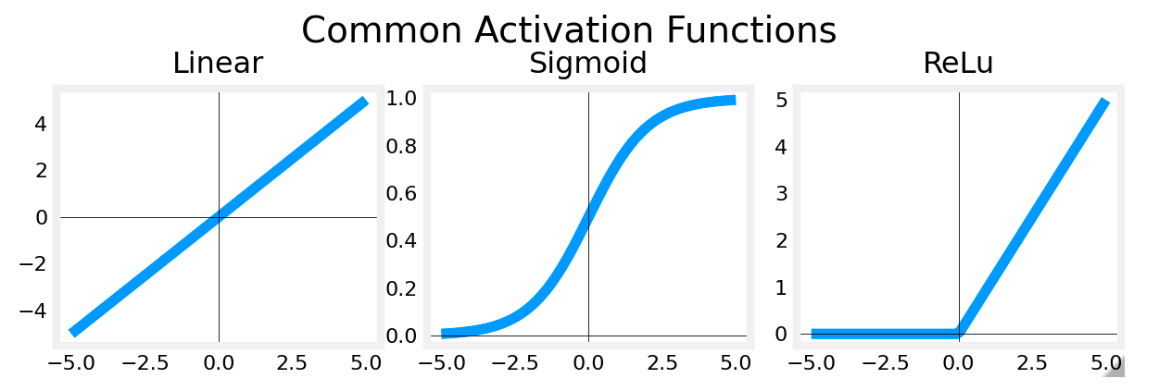
# 激活函数# ReLUg ( z ) = m a x ( 0 , z ) g(z)=max(0,z)
g ( z ) = m a x ( 0 , z )
# sigmoidg ( z ) = 1 1 + e − z g(z)=\frac{1}{1+e^{-z}}
g ( z ) = 1 + e − z 1
# linear 激活函数g ( z ) = z g(z)=z
g ( z ) = z
sigmoid 最适合 on/off 或 binary 情况。ReLU 提供连续的线性关系。此外,它有一个 ‘off’ 范围,其中 output 为零。“off” 功能使 ReLU 成为 Non-Linear 激活。
output layer
正值的回归 -relu
binary 分类 - sigmoid
linear - 回归
hidden layer
ReLU 大部分
sigmoid 分类
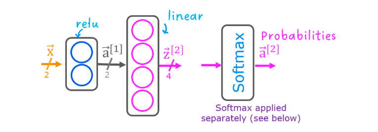
# softmax regression在具有 Softmax 输出的 softmax 回归和神经网络中,都会生成 N 个输出,并选择 1 个输出作为预测类别。在这两种情况下,向量 𝐳 都是由线性函数生成的,该函数应用于 softmax 函数。softmax 函数转换为 𝐳 概率分布,应用 softmax 后,每个输出将介于 0 和 1 之间,并且输出将加到 1,以便可以将其解释为概率。较大的输入将对应于较大的输出概率。
a_j = \frac{e^{z_j}}{\sum_{k = 1}^{N}e^{z_k}} = P(y = j|\vec{x})$$,即假如有10个输出,此时N=10,那么$$a_1 = \frac{e^{z_1}}{(e^{z_1}+\cdots+e^{z_{10}})} = P(y = 1|\vec{x})
输出 𝐚是一个长度为 N 的向量
\begin{align} \mathbf{a}(x) = \begin{bmatrix} P(y = 1 | \mathbf{x}; \mathbf{w},b) \\ \vdots \\ P(y = N | \mathbf{x}; \mathbf{w},b) \end{bmatrix} = \frac{1}{ \sum_{k=1}^{N}{e^{z_k} }} \begin{bmatrix} e^{z_1} \\ \vdots \\ e^{z_{N}} \\ \end{bmatrix} \end{align}
输出是概率向量,第一个条目是给定输入 𝐱 和参数 𝐰 以及 𝐛 的输入是第一个类别的概率
N=2 时,变为 Logistic regression,即 softmax regression 是 Logistic regression 的广义形式
# softmax Cost functionsoftmax 损失函数是 cross-entropy loss$$\begin {align} \ &\text {loss}(a_1,\cdots,a_N,y)= \begin {cases} -\log a_1 & \text {if } y = 1 \ -\log a_2 & \text {if } y = 2 \ \vdots & \ -\log a_N & \text {if } y = N \end {cases} \end {align} $$
其中 y 是此示例的目标类别, 𝐚 是 softmax 函数的输出。 a 的概率总和为 1
J ( w , b ) = − 1 m [ ∑ i = 1 m ∑ j = 1 N 1 { y ( i ) = = j } log e z j ( i ) ∑ k = 1 N e z k ( i ) ] J(\mathbf{w},b) = -\frac{1}{m} \left[ \sum_{i=1}^{m} \sum_{j=1}^{N} 1\left\{y^{(i)} == j\right\} \log \frac{e^{z^{(i)}_j}}{\sum_{k=1}^N e^{z^{(i)}_k} }\right]
J ( w , b ) = − m 1 [ i = 1 ∑ m j = 1 ∑ N 1 { y ( i ) = = j } log ∑ k = 1 N e z k ( i ) e z j ( i ) ]
softmax output
a ⃗ [ 3 ] = ( a 1 [ 3 ] , ⋯ , a 10 [ 3 ] ) = g ( z 1 [ 3 ] , ⋯ , z 10 [ 3 ] ) \vec{a}^{[3]} = \left(a_1^{[3]},\cdots,a_{10}^{[3]}\right) = g\left(z_1^{[3]},\cdots,z_{10}^{[3]}\right)
a [ 3 ] = ( a 1 [ 3 ] , ⋯ , a 1 0 [ 3 ] ) = g ( z 1 [ 3 ] , ⋯ , z 1 0 [ 3 ] )
此时损失函数称为
SparseCategoricalCrossentropy
# Tensorflow 中实现 softmax 交叉熵损失使用 softmax 作为最终 Dense 层中的激活实现的
1 2 3 4 5 6 7 8 9 10 11 12 13 14 15 16 17 18 19 20 21 22 23 24 25 26 27 model = Sequential( [ Dense(25 , activation = 'relu' ), Dense(15 , activation = 'relu' ), Dense(4 , activation = 'softmax' ) ] ) model.compile ( loss=tf.keras.losses.SparseCategoricalCrossentropy(), optimizer=tf.keras.optimizers.Adam(0.001 ), ) model.fit( X_train,y_train, epochs=10 ) p_nonpreferred = model.predict(X_train) print (p_nonpreferred [:2 ])print ("largest value" , np.max (p_nonpreferred), "smallest value" , np.min (p_nonpreferred))''' [[7.95e-04 4.70e-03 9.74e-01 2.01e-02] [9.95e-01 5.41e-03 5.92e-05 2.75e-06]] largest value 1.0 smallest value 1.7346442e-11 '''
将 softmax 和 loss 结合起来,可以获得更稳定、更准确的结果。
1 2 3 4 5 6 7 8 9 10 11 12 13 14 15 16 17 18 19 20 21 22 23 24 25 26 27 28 29 30 31 32 33 34 35 36 37 38 39 40 41 42 43 44 45 46 47 48 49 50 51 52 preferred_model = Sequential( [ Dense(25 , activation = 'relu' ), Dense(15 , activation = 'relu' ), Dense(4 , activation = 'linear' ) ] ) preferred_model.compile ( loss=tf.keras.losses.SparseCategoricalCrossentropy(from_logits=True ), optimizer=tf.keras.optimizers.Adam(0.001 ), ) preferred_model.fit( X_train,y_train, epochs=10 ) p_preferred = preferred_model.predict(X_train) print (f"two example output vectors:\n {p_preferred[:2 ]} " )print ("largest value" , np.max (p_preferred), "smallest value" , np.min (p_preferred))''' two example output vectors: [[-2.28 -2.71 3.53 -0.2 ] [ 4.81 -0.54 -4.27 -5.81]] largest value 10.816914 smallest value -11.811311 ''' sm_preferred = tf.nn.softmax(p_preferred).numpy() print (f"two example output vectors:\n {sm_preferred[:2 ]} " )print ("largest value" , np.max (sm_preferred), "smallest value" , np.min (sm_preferred))''' two example output vectors: [[2.90e-03 1.88e-03 9.72e-01 2.33e-02] [9.95e-01 4.73e-03 1.13e-04 2.43e-05]] largest value 0.9999976 smallest value 4.1457393e-10 ''' for i in range (5 ): print ( f"{p_preferred[i]} , category: {np.argmax(p_preferred[i])} " ) ''' [-2.28 -2.71 3.53 -0.2 ], category: 2 [ 4.81 -0.54 -4.27 -5.81], category: 0 [ 3.47 0.05 -3.17 -4.48], category: 0 [-0.61 4.43 -1.14 -1.07], category: 1 [ 0.02 -4.27 4.9 -3.78], category: 2 '''
# 多类神经网络通常用于对数据进行分类。例如拍摄照片并将照片中的主体分类为
这种类型的网络在其最后一层中将有多个单元。每个输出都与一个类别相关联。将输入示例应用于网络时,具有最高值的输出是预测的类别。如果输出应用于 softmax 函数,则 softmax 的输出将提供输入在每个类别中的概率。
输出层使用的是 linear 而不是 softmax activation。虽然可以在输出层中包含 softmax,但如果在训练期间将线性输出传递给损失函数,它在数值上会更加稳定。
1 2 3 4 5 6 7 8 9 10 11 12 13 14 15 16 17 18 19 20 21 22 23 24 25 26 27 28 29 30 31 32 33 34 tf.random.set_seed(1234 ) model = Sequential( [ Dense(2 , activation = 'relu' , name = "L1" ), Dense(4 , activation = 'linear' , name = "L2" ) ] ) model.compile ( loss=tf.keras.losses.SparseCategoricalCrossentropy(from_logits=True ), optimizer=tf.keras.optimizers.Adam(0.01 ), ) model.fit( X_train,y_train, epochs=200 ) plt_cat_mc(X_train, y_train, model, classes) l1 = model.get_layer("L1" ) W1,b1 = l1.get_weights() plt_layer_relu(X_train, y_train.reshape(-1 ,), W1, b1, classes) l2 = model.get_layer("L2" ) W2, b2 = l2.get_weights() Xl2 = np.maximum(0 , np.dot(X_train,W1) + b1) plt_output_layer_linear(Xl2, y_train.reshape(-1 ,), W2, b2, classes, x0_rng = (-0.25 ,np.amax(Xl2[:,0 ])), x1_rng = (-0.25 ,np.amax(Xl2[:,1 ])))
# Adam对于每个 w,都有自己的学习率。使梯度下降更快
# layer types# Dense layer# convolutional layer卷积层,每个神经元只查看图像中的一部分
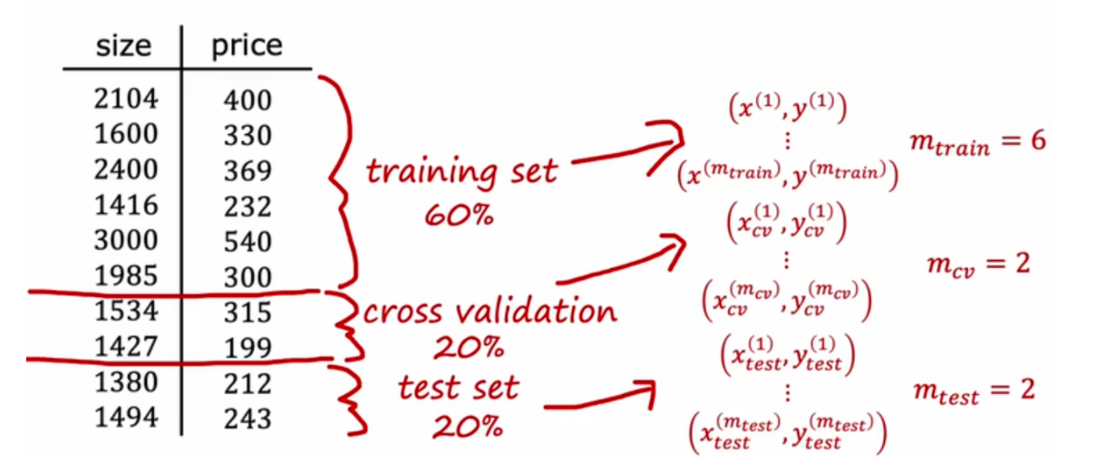
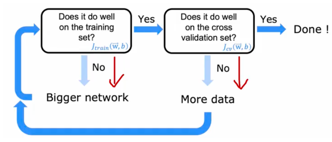
# 模型评估拆分数据为训练集 (training set) 和测试集 (test set) 和交叉验证集 cross validation /dev set
( x ( m t r a i n ) , y m t r a i n ) (x^{(m_{train})},y^{m_{train}})
( x ( m t r a i n ) , y m t r a i n )
( x t e s t ( m t e s t ) , y t e s t ( m t e s t ) ) (x_{test}^{(m_{test})},y_{test}^{(m_{test})})
( x t e s t ( m t e s t ) , y t e s t ( m t e s t ) )
( x c v ( m c v ) , y c v ( m c v ) ) (x_{cv}^{(m_{cv})},y_{cv}^{(m_{cv})})
( x c v ( m c v ) , y c v ( m c v ) )
训练集
交叉验证集(也称为验证、开发或开发集)
测试集
cost function of linear regression
J ( w ⃗ , b ) = min w ⃗ , b [ 1 2 m train ∑ i = 1 m train ( f w ⃗ , b ( x ⃗ ( i ) ) − y ( i ) ) 2 + λ 2 m train ∑ j = 1 n w j 2 ] J(\vec{w},b) = \min_{\vec{w},b}\left[\frac{1}{2m_{\text{train}}}\sum_{i = 1}^{m_{\text{train}}}(f_{\vec{w},b}(\vec{x}^{(i)) - y^{(i)})^2} + \frac{\lambda}{2m_{\text{train}}}\sum_{j = 1}^{n} w_j^2\right]
J ( w , b ) = w , b min [ 2 m train 1 i = 1 ∑ m train ( f w , b ( x ( i ) ) − y ( i ) ) 2 + 2 m train λ j = 1 ∑ n w j 2 ]
test error
J test ( w ⃗ , b ) = 1 2 m test [ ∑ i = 1 m test ( f w ⃗ , b ( x ⃗ test ( i ) ) − y test ( i ) ) 2 ] J_{\text{test}}(\vec{w},b) = \frac{1}{2m_{\text{test}}}\left[\sum_{i = 1}^{m_{\text{test}}}\left(f_{\vec{w},b}(\vec{x}^{(i)}_{\text{test}}) - y^{(i)}_{\text{test}}\right)^2\right]
J test ( w , b ) = 2 m test 1 [ i = 1 ∑ m test ( f w , b ( x test ( i ) ) − y test ( i ) ) 2 ]
training error
J train ( w ⃗ , b ) = 1 2 m train [ ∑ i = 1 m train ( f w ⃗ , b ( x ⃗ train ( i ) ) − y train ( i ) ) 2 ] J_{\text{train}}(\vec{w},b) = \frac{1}{2m_{\text{train}}}\left[\sum_{i = 1}^{m_{\text{train}}}\left(f_{\vec{w},b}(\vec{x}^{(i)}_{\text{train}}) - y^{(i)}_{\text{train}}\right)^2\right]
J train ( w , b ) = 2 m train 1 [ i = 1 ∑ m train ( f w , b ( x train ( i ) ) − y train ( i ) ) 2 ]
overfit 的状态,jtrain 将会很小。jtest 将会很高
cost function of classification
J ( w ⃗ , b ) = − 1 m ∑ i = 1 m [ y ( i ) log ( f w ⃗ , b ( x ⃗ ( i ) ) ) + ( 1 − y ( i ) ) log ( 1 − f w ⃗ , b ( x ⃗ ( i ) ) ) ] + λ 2 m ∑ j = 1 n w j 2 J(\vec{w},b)=-\frac{1}{m}\sum_{i = 1}^{m}\left[y^{(i)}\log\left(f_{\vec{w},b}(\vec{x}^{(i)})\right)+(1 - y^{(i)})\log\left(1 - f_{\vec{w},b}(\vec{x}^{(i)})\right)\right]+\frac{\lambda}{2m}\sum_{j = 1}^{n}w_j^2
J ( w , b ) = − m 1 i = 1 ∑ m [ y ( i ) log ( f w , b ( x ( i ) ) ) + ( 1 − y ( i ) ) log ( 1 − f w , b ( x ( i ) ) ) ] + 2 m λ j = 1 ∑ n w j 2
compute test error
J test ( w ⃗ , b ) = − 1 m test ∑ i = 1 m test [ y test ( i ) log ( f w ⃗ , b ( x ⃗ test ( i ) ) ) + ( 1 − y test ( i ) ) log ( 1 − f w ⃗ , b ( x ⃗ test ( i ) ) ) ] J_{\text{test}}(\vec{w},b)=-\frac{1}{m_{\text{test}}}\sum_{i = 1}^{m_{\text{test}}}\left[y^{(i)}_{\text{test}}\log\left(f_{\vec{w},b}(\vec{x}^{(i)}_{\text{test}})\right)+(1 - y^{(i)}_{\text{test}})\log\left(1 - f_{\vec{w},b}(\vec{x}^{(i)}_{\text{test}})\right)\right]
J test ( w , b ) = − m test 1 i = 1 ∑ m test [ y test ( i ) log ( f w , b ( x test ( i ) ) ) + ( 1 − y test ( i ) ) log ( 1 − f w , b ( x test ( i ) ) ) ]
compute train error
J train ( w ⃗ , b ) = − 1 m train ∑ i = 1 m train [ y train ( i ) log ( f w ⃗ , b ( x ⃗ train ( i ) ) ) + ( 1 − y train ( i ) ) log ( 1 − f w ⃗ , b ( x ⃗ train ( i ) ) ) ] J_{\text{train}}(\vec{w},b)=-\frac{1}{m_{\text{train}}}\sum_{i = 1}^{m_{\text{train}}}\left[y^{(i)}_{\text{train}}\log\left(f_{\vec{w},b}(\vec{x}^{(i)}_{\text{train}})\right)+(1 - y^{(i)}_{\text{train}})\log\left(1 - f_{\vec{w},b}(\vec{x}^{(i)}_{\text{train}})\right)\right]
J train ( w , b ) = − m train 1 i = 1 ∑ m train [ y train ( i ) log ( f w , b ( x train ( i ) ) ) + ( 1 − y train ( i ) ) log ( 1 − f w , b ( x train ( i ) ) ) ]
fraction of the test set and the fraction of the train set that the algorithm has misclassified.
y ^ = { 1 if f w ⃗ , b ( x ⃗ ( i ) ) ≥ 0.5 0 if f w ⃗ , b ( x ⃗ ( i ) ) < 0.5 \hat{y}= \begin{cases} 1 & \text{if } f_{\vec{w},b}(\vec{x}^{(i)})\geq0.5 \\ 0 & \text{if } f_{\vec{w},b}(\vec{x}^{(i)})<0.5 \end{cases}
y ^ = { 1 0 if f w , b ( x ( i ) ) ≥ 0 . 5 if f w , b ( x ( i ) ) < 0 . 5
count $$\hat{y}\neq y$$
J_{\text{test}}(\vec{w},b) $$ is the fraction of the test set that has been misclassified.
$$J_{\text{train}}(\vec{w},b) $$is the fraction of the train set that has been misclassified.
training error $$ J_{\text{train}}(\vec{w},b) = \frac{1}{2m_{\text{train}}}\left[\sum_{i = 1}^{m_{\text{train}}}\left(f_{\vec{w},b}(\vec{x}^{(i)}) - y^{(i)}\right)^2\right]
cross validation error $$ J_cv}(\vec{w},b) = \frac{1}{2m_{cv}}\left[\sum_{i = 1}【 {m_{cv 】 }\left(f_\vec{w},b}(\vec{x}【 {(i) 】 cv}) - y【 {(i) 】
test error $$ J_\text{test}}(\vec{w},b) = \frac{1}{2m_{\text{test}}}\left[\sum_{i = 1}【 {m_{\text{test 】 }}\left(f_\vec{w},b}(\vec{x}【 {(i) 】 \text{test}}) - y【 {(i) 】
cross vadidation 决定那个模型更适合,test 评估泛化误差估计值
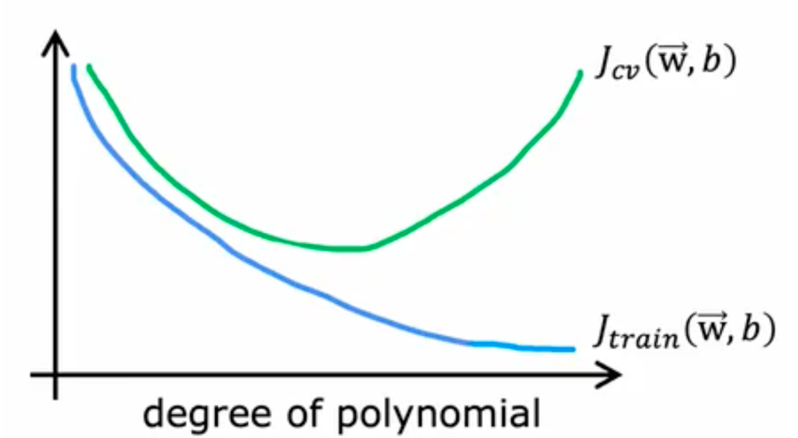
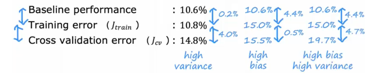
# bias variance高方差 : Jcv >> jtrain,此时 overfit
高偏差:jcv,jtrain 都很高,此时,此时 underfit
高方差 & 高偏差:jtrain high,jcv >> jtrain, 此时部分 overfit,部分 underfit
要解决高偏差问题,:
try adding polynomial features 尝试添加多项式特征
try getting additional features 尝试获取其他功能
try decreasing the regularization parameter 尝试减小 正则化 参数
To fix a high variance problem, you can:
要解决高方差问题,您可以:
try increasing the regularization parameter 尝试增加 正则化 参数
try smaller sets of features
get more training examples 获取更多训练集
目标:jtrain&jcv 都很低
# 正则化后偏差和方差f w ⃗ , b ( x ) = w 1 x + w 2 x 2 + w 3 x 3 + w 4 x 4 + b f_{\vec{w},b}(x) = w_1x + w_2x^2 + w_3x^3 + w_4x^4 + b
f w , b ( x ) = w 1 x + w 2 x 2 + w 3 x 3 + w 4 x 4 + b
J ( w ⃗ , b ) = 1 2 m ∑ i = 1 m ( f w ⃗ , b ( x ⃗ ( i ) ) − y ( i ) ) 2 + λ 2 m ∑ j = 1 n w j 2 \\ J(\vec{w},b) = \frac{1}{2m}\sum_{i = 1}^{m}\left(f_{\vec{w},b}(\vec{x}^{(i)}) - y^{(i)}\right)^2 + \frac{\lambda}{2m}\sum_{j = 1}^{n}w_j^2
J ( w , b ) = 2 m 1 i = 1 ∑ m ( f w , b ( x ( i ) ) − y ( i ) ) 2 + 2 m λ j = 1 ∑ n w j 2
基线表现和 traning error 差值可以决定是否存在 high bias
Jtrain 和 Jcv 之间差值可以决定是否存在 high variance
baseline 选取方式
Human level performance
Competing algorithms performance
Guess based on experience
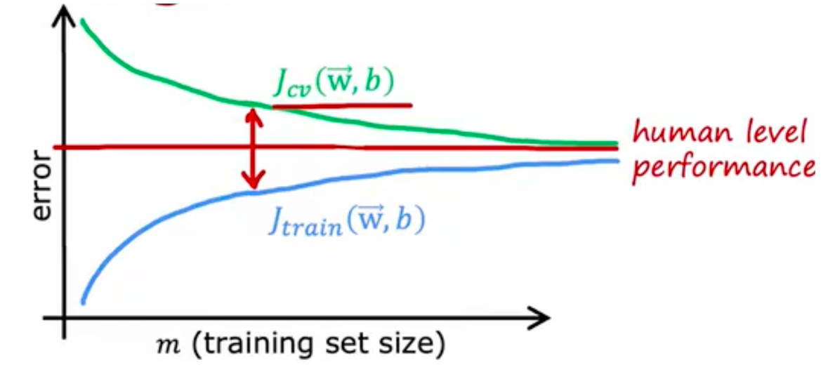
# learning curveshigh bias
增加训练数据对于这种情况用处不大
high variance
此时获取更多训练数据是有用的
正则化线性回归对于大的 Jwb 解决
Get more training examples fixes high variance
Try smaller sets of features fix high variance
Try getting additional features fix high bias
Try adding polynomial features fix high bias
Try decreasing $$\lambda$$ fix high bias
Try increasing $$\lambda$$ fix high variance
减少训练集无法修正 high bias
当经过合适正则化的大型神经网络,通常会表现的和较小的一样甚至更好
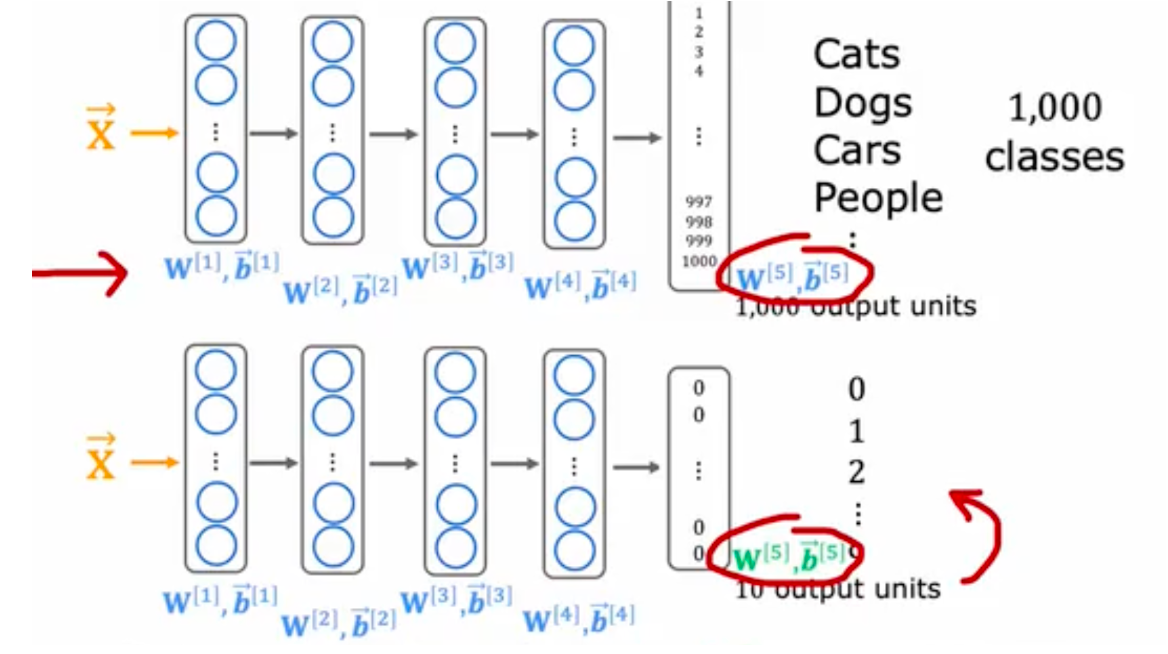
# error analysis# add data# transfer learning先在大型数据集上训练,然后在较小的数据集上进一步调整参数
用上图的 w1,b1 到 w4,b4 迁移到 下图的 w1,b1 到 w4,b4 ,但是对于 w5b5 重新调整
对 pre-train 模型进行 fine-tuning
1、下载在具有相同输入的大型数据集上预训练神经网络参数,或者自己训练一个。但输入类型必须相同 (图像,声音,文本)
2、在自己的数据上进一步训练或微调
# 数据倾斜precision:(of all patients where we predicted y = 1, what fraction actually has the rare disease?)
True positives # p r e d i c t e d P o s i t i v e = True positives True pos + False pos = 15 15 + 5 \frac{\text{True positives}}{\#predicted Positive} \text{=} \frac{\text{True positives}}{\text{True pos + False pos}} = \frac{15}{15+5}
# p r e d i c t e d P o s i t i v e True positives = True pos + False pos True positives = 1 5 + 5 1 5
recall: (of all patients that actually have the rare disease, what fraction did we correctly detect as having it?) 可以检测学习算法是否总是预测 0
True positives #actual Positive = True positives True pos + False neg = 15 15 + 10 \frac{\text{True positives}}{\text{\#actual Positive}} \text{=} \frac{\text{True positives}}{\text{True pos + False neg}} = \frac{15}{15+10}
#actual Positive True positives = True pos + False neg True positives = 1 5 + 1 0 1 5
保证 recall 和 precision 都比较高,来证明算法生效
预测 Logistic regression 时,提高预测为 1 的阈值,会导致 precision 提高,但是 recall 降低
F1 Score = $$2\frac {PR}{P+R}$$, 也称为调和平均
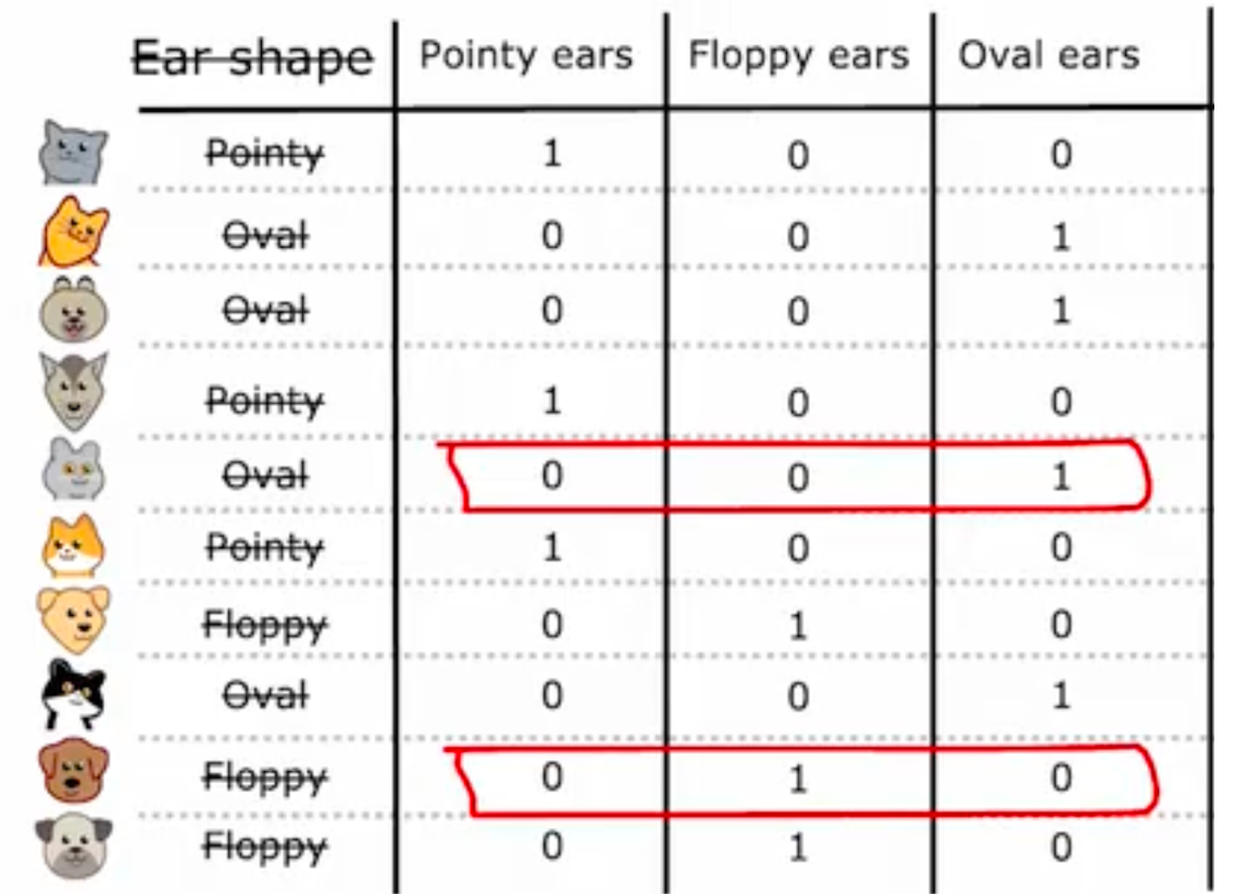
# 决策树root node / decision node / leaf node
决策 1:如何选择在每个节点上依据哪个特征进行划分?
使纯度最大化(或使不纯度最小化)
决策 2 :何时停止划分?
当一个节点完全属于某一个类别时
当划分一个节点会导致树的深度超过最大深度时
当纯度得分的提升低于某个阈值时
当一个节点中的样本数量低于某个阈值时
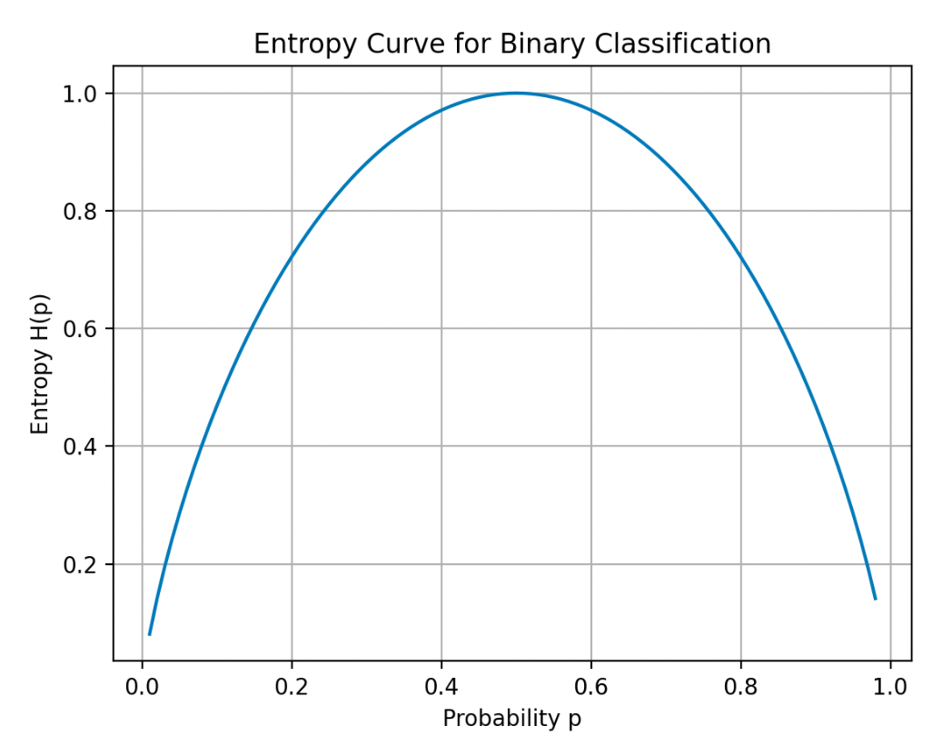
entropy function
衡量数据集中杂质
H(p1)
p 0 = 1 − p 1 H ( p 1 ) = − p 1 log 2 ( p 1 ) − p 0 log 2 ( p 0 ) = − p 1 log 2 ( p 1 ) − ( 1 − p 1 ) log 2 ( 1 − p 1 ) p_0 = 1 - p_1 \\ H(p_1) = -p_1\log_2(p_1) - p_0\log_2(p_0)= -p_1\log_2(p_1) - (1 - p_1)\log_2(1 - p_1)
p 0 = 1 − p 1 H ( p 1 ) = − p 1 log 2 ( p 1 ) − p 0 log 2 ( p 0 ) = − p 1 log 2 ( p 1 ) − ( 1 − p 1 ) log 2 ( 1 − p 1 )
# 信息增益减少 entropy
计算加权平均
上图中 0.28 是信息增益最多的,所以在 root node 选择 ear
\text{Information Gain} = H(p_1^{\text{root}}) - \left(w^{\text{left}}H(p_1^{\text{left}}) + w^{\text{right}}H(p_1^{\text{right}})\right)$$,其中$$H(p_1) = -p_1\log_2(p_1) - p_0\log_2(p_0)= -p_1\log_2(p_1) - (1 - p_1)\log_2(1 - p_1)
这是计算决策树中信息增益(或类似增益指标)的公式 。其中:
公式通过父节点熵减去子节点加权熵和,得到分裂前后的熵变化,用于评估特征分裂的优劣,值越大表示分裂后数据不确定性降低越多,分裂效果越好 。
# one-hot encoding如果特征中有 k 个值,可以创建 k 个二元特征来替换他
# 分割连续值对于指定阈值进行分割
# regression tree预测数值,不再是分类
选择加权方差最低的值
# tree ensemble
# 放回抽样# XGboost# boosted tree intuitionGiven training set of size $$$$
For $$b = $$ to B:
Use sampling with replacement to create a new training set of size $$$$
But instead of picking from all examples with equal $$(1/m$$ probability, make it more likely to pick examples that the previously trained trees misclassify
Train a decision tree on the new dataset
1
2
3
4
5
6
7
8
from xgboost import XGBClassifiermodel = XGBClassifier() model.fit(X_train, y_train) y_pred = model.predict(X_test) from xgboost import XGBRegressormodel = XGBRegressor() model.fit(X_train, y_train) y_pred = model.predict(X_test)
# 决策树 / 神经网络决策树:适合处理结构化数据,训练更快,小决策树更容易理解,使用树时,最好用 XGboost
神经网络:所有数据都很好,包含结构化和非结构化。比决策树训练更慢。可以迁移学习。适合构建更大的模型。当构建一个由多个模型协同工作的系统时,将多个神经网络串联起来可能会更容易。
# 无监督学习# k-means1、确定 cluster centroids
2、分配每个点到簇质心
3、将所以点取平均值,将质心移到到这里
4、重新关联点和质心
5、重复,直到质心不再发生变化,点也不再发生变化
(c^{(i)} =) $$index of cluster (1, 2, ..., K)to which example $$(x^{(i)})$$ is currently assigned
$$(\mu_k =) $$cluster centroid k
$$(\mu_{c^{(i)}} =)$$ cluster centroid of cluster to which example $$(x^{(i)}) $$has been assigned
$$ J(c^{(1)}, ..., c^{(m)}, \mu_1, ..., \mu_K) = \frac{1}{m}\sum_{i = 1}^{m}\lVert x^{(i)} - \mu_{c^{(i)}}\rVert^2
多次运行 kmeans,计算每个 cost function,找到最小的 cost
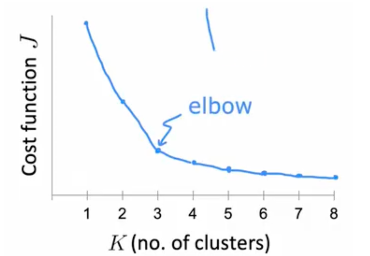
选择 K 值
ELBO:选择不同的 k 值运行,并计算 cost function
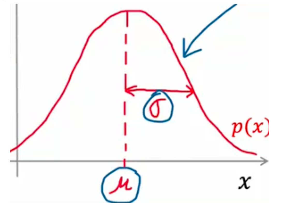
# 异常检测正态分布 $$P (x)=\frac1}{\sqrt{2\pi\sigma【 {2 】 }}e^-\frac{(x - \mu)【 {2 】 }2\sigma【 {2 】 }}$$
σ 2 = 1 m ∑ i = 1 m ( x i − μ ) 2 \sigma^{2}=\frac{1}{m}\sum_{i = 1}^{m}(x_{i}-\mu)^{2}
σ 2 = m 1 i = 1 ∑ m ( x i − μ ) 2
μ = 1 m ∑ i = 1 m x i \mu =\frac{1}{m}\sum_{i = 1}^{m}x^{i}
μ = m 1 i = 1 ∑ m x i
1、选定特征 Xi
3、计算 $$\sigma^{2}$$ 和 $$\mu$$
3、$$ p(x) = \prod_j=1}【 {n 】 p(x_j; \mu_j, \sigma_j^2) = \prod_j=1}【 {n 】 \frac1}{\sqrt{2\pi}\sigma_j} \exp\left(-\frac{(x_j - \mu_j)【 2 】 2\sigma_j【 2 】 \right)$$
4、 判断 $$p (x)<\varepsilon$$, 如果是,标记为异常
real-number 评估
创建 CVset test set
100000 good (normal) engines
20 flawed engines (anomalous)
Training set: 6000 good engines
CV: 2000 good engines (y = 0), 10 anomalous (y = 1)
Test: 2000 good engines (y = 0), 10 anomalous (y = 1)
Alternative:
Training set: 6000 good engines
CV: 4000 good engines (y = 0), 20 anomalous (y = 1)
No test set
p (x) 是 training set,On a cross validation/test example x, predict
y = { 1 if p ( x ) < ε (anomaly) 0 if p ( x ) ≥ ε (normal) y=\begin{cases} 1 & \text{if } p(x)<\varepsilon \text{ (anomaly)}\\ 0 & \text{if } p(x)\geq\varepsilon \text{ (normal)} \end{cases}
y = { 1 0 if p ( x ) < ε (anomaly) if p ( x ) ≥ ε (normal)
# 监督学习 / 异常检测异常检测:
极少数正例(y = 1)。(0-20 很常见)。大量反面例子(y = 0)。
存在许多不同的异常,异常的 "类型" 多种多样。任何算法都很难从正面例子中了解异常情况是什么样的;未来的异常情况可能与我们目前看到的异常例子完全不同。
欺诈检测、从未见过的缺陷,发现黑客入侵
监督学习:
大量正例和反例
足够多的正面示例,让算法了解正面示例是什么样的,未来的正面示例可能与训练集中的示例相似。
垃圾邮件检测、发现已知的缺陷,疾病分类,天气预测
# 特征选择转换特征,使其变为高斯分布,比如使用 $$log_2,log (x+1),x^{\frac {1}{2}}$$
特征转换时,需要转换 cv 和 test set
误差分析:
增加其他特征,比如一些已知特征的组合,来使 p (x) 足够大
# 推荐算法# notation
n_u$$ 用户数量
$$n_m$$电影数量
$$r(i,j)=1$$用户j已经对电影i做了评分
$$y^{(i,j)}$$用户j给电影i的评分
n 特征数目
$$x^{(1)} $$第一部电影的特征向量 $$[0.9,0]
{w^{(j)}} \cdot {x^{(i)}}+b^{(j)}$$ 预测用户j给电影i的评分
$$m^{(j)} $$用户评分的电影总数
| Movie | Alice(1) | Bob(2) | Carol(3) | Dave(4) | $$(x_1) (romance)$$ | $$(x_2) (action)$$ |
| -------------------- | -------- | ------ | -------- | ------- | ------------------- | ------------------ |
| Love at last | 5 | 5 | 0 | 0 | 0.9 | 0 |
| Romance forever | 5 | ? | ? | 0 | 1.0 | 0.01 |
| Cute puppies of love | ? | 4 | 0 | ? | 0.99 | 0 |
| Nonstop car chases | 0 | 0 | 5 | 4 | 0.1 | 1.0 |
| Swords vs. karate | 0 | 0 | 5 | ? | 0 | 0.9 |
#### cost function
学习用户j的wj,bj
$$ \min_{w^{(j)},b^{(j)}}J(w^{(j)},b^{(j)}) = \frac{1}{2m^{(j)}}\sum_{i:r(i,j)=1}(w^{(j)}\cdot x^{(i)} + b^{(j)} - y^{(i,j)})^2+\frac{\lambda}{2m^{(j)}}\sum_{k = 1}^{n}(w_k^{(j)})^2
学习所有用的 wi,bi
J ( w ( 1 ) , … , w ( n u ) b ( 1 ) , … , b ( n u ) ) = 1 2 ∑ j = 1 n u ∑ i : r ( i , j ) = 1 ( w ( j ) ⋅ x ( i ) + b ( j ) − y ( i , j ) ) 2 + λ 2 ∑ j = 1 n u ∑ k = 1 n ( w k ( j ) ) 2 J\left(\begin{matrix} w^{(1)}, \ldots, w^{(n_u)} \\ b^{(1)}, \ldots, b^{(n_u)} \end{matrix}\right)=\frac{1}{2}\sum_{j = 1}^{n_u}\sum_{i:r(i,j)=1}(w^{(j)}\cdot x^{(i)} + b^{(j)} - y^{(i,j)})^2+\frac{\lambda}{2}\sum_{j = 1}^{n_u}\sum_{k = 1}^{n}(w_k^{(j)})^2
J ( w ( 1 ) , … , w ( n u ) b ( 1 ) , … , b ( n u ) ) = 2 1 j = 1 ∑ n u i : r ( i , j ) = 1 ∑ ( w ( j ) ⋅ x ( i ) + b ( j ) − y ( i , j ) ) 2 + 2 λ j = 1 ∑ n u k = 1 ∑ n ( w k ( j ) ) 2
Cost function
to learn $$(x^{(i)})$$
J ( x ( i ) ) = 1 2 ∑ j : r ( i , j ) = 1 ( w ( j ) ⋅ x ( i ) + b ( j ) − y ( i , j ) ) 2 + λ 2 ∑ k = 1 n ( x k ( i ) ) 2 J(x^{(i)}) = \frac{1}{2}\sum_{j:r(i,j)=1}(w^{(j)}\cdot x^{(i)} + b^{(j)} - y^{(i,j)})^2+\frac{\lambda}{2}\sum_{k = 1}^{n}(x_k^{(i)})^2
J ( x ( i ) ) = 2 1 j : r ( i , j ) = 1 ∑ ( w ( j ) ⋅ x ( i ) + b ( j ) − y ( i , j ) ) 2 + 2 λ k = 1 ∑ n ( x k ( i ) ) 2
To learn$$ (x^(1)}, x【 {(2) 】 , \cdots, x^{(n_m)})$$
J ( x ( 1 ) , x ( 2 ) , ⋯ , x ( n m ) ) = 1 2 ∑ i = 1 n m ∑ j : r ( i , j ) = 1 ( w ( j ) ⋅ x ( i ) + b ( j ) − y ( i , j ) ) 2 + λ 2 ∑ i = 1 n m ∑ k = 1 n ( x k ( i ) ) 2 J(x^{(1)}, x^{(2)}, \cdots, x^{(n_m)}) = \frac{1}{2}\sum_{i = 1}^{n_m}\sum_{j:r(i,j)=1}(w^{(j)}\cdot x^{(i)} + b^{(j)} - y^{(i,j)})^2+\frac{\lambda}{2}\sum_{i = 1}^{n_m}\sum_{k = 1}^{n}(x_k^{(i)})^2
J ( x ( 1 ) , x ( 2 ) , ⋯ , x ( n m ) ) = 2 1 i = 1 ∑ n m j : r ( i , j ) = 1 ∑ ( w ( j ) ⋅ x ( i ) + b ( j ) − y ( i , j ) ) 2 + 2 λ i = 1 ∑ n m k = 1 ∑ n ( x k ( i ) ) 2
# 协同过滤多个用户评估一部电影,这种协同反馈可以了解电影特点。预测未对同一部电影评分的用户在未来如何评分
min w ( 1 ) , … , w ( n u ) b ( 1 ) , … , b ( n u ) x ( 1 ) , … , x ( n m ) J ( w , b , x ) = 1 2 ∑ ( i , j ) : r ( i , j ) = 1 ( w ( j ) ⋅ x ( i ) + b ( j ) − y ( i , j ) ) 2 + λ 2 ∑ j = 1 n u ∑ k = 1 n ( w k ( j ) ) 2 + λ 2 ∑ i = 1 n m ∑ k = 1 n ( x k ( i ) ) 2 \min_{\substack{ w^{(1)}, \ldots, w^{(n_u)} \\ b^{(1)}, \ldots, b^{(n_u)} \\ x^{(1)}, \ldots, x^{(n_m)} }}J(w, b, x) = \frac{1}{2}\sum_{(i,j):r(i,j)=1}(w^{(j)}\cdot x^{(i)} + b^{(j)} - y^{(i,j)})^2+\frac{\lambda}{2}\sum_{j = 1}^{n_u}\sum_{k = 1}^{n}(w_k^{(j)})^2+\frac{\lambda}{2}\sum_{i = 1}^{n_m}\sum_{k = 1}^{n}(x_k^{(i)})^2
w ( 1 ) , … , w ( n u ) b ( 1 ) , … , b ( n u ) x ( 1 ) , … , x ( n m ) min J ( w , b , x ) = 2 1 ( i , j ) : r ( i , j ) = 1 ∑ ( w ( j ) ⋅ x ( i ) + b ( j ) − y ( i , j ) ) 2 + 2 λ j = 1 ∑ n u k = 1 ∑ n ( w k ( j ) ) 2 + 2 λ i = 1 ∑ n m k = 1 ∑ n ( x k ( i ) ) 2
梯度下降
repeat {
\begin{align} w_i^{(j)} &= w_i^{(j)}-\alpha\frac{\partial}{\partial w_i^{(j)}}J(w, b, x)\\ b^{(j)} &= b^{(j)}-\alpha\frac{\partial}{\partial b^{(j)}}J(w, b, x)\\ x_k^{(i)} &= x_k^{(i)}-\alpha\frac{\partial}{\partial x_k^{(i)}}J(w, b, x) \end{align}
}
# 二元标签评分的含义:
1 - 展示项目后参与
0 - 展示项目后未参与。
? - 尚未展示项目
Predict that the probability of $$(y^(i,j)} = 1)$$ is given by $$(g(w【 {(j) 】 \cdot x^(i)} + b【 {(j) 】 ))$$
where $$(g(z)=\frac1}{1 + e【 {-z 】 }) $$
cost function
Loss for binary labels$$ (y^{(i,j)})$$:
f ( w , b , x ) ( x ) = g ( w ( j ) ⋅ x ( i ) + b ( j ) ) f_{(w,b,x)}(x)=g(w^{(j)}\cdot x^{(i)} + b^{(j)})
f ( w , b , x ) ( x ) = g ( w ( j ) ⋅ x ( i ) + b ( j ) )
L ( f ( w , b , x ) ( x ) , y ( i , j ) ) = − y ( i , j ) log ( f ( w , b , x ) ( x ) ) − ( 1 − y ( i , j ) ) log ( 1 − f ( w , b , x ) ( x ) ) L(f_{(w,b,x)}(x), y^{(i,j)})=-y^{(i,j)}\log(f_{(w,b,x)}(x))-(1 - y^{(i,j)})\log(1 - f_{(w,b,x)}(x))
L ( f ( w , b , x ) ( x ) , y ( i , j ) ) = − y ( i , j ) log ( f ( w , b , x ) ( x ) ) − ( 1 − y ( i , j ) ) log ( 1 − f ( w , b , x ) ( x ) )
J ( w , b , x ) = ∑ ( i , j ) : r ( i , j ) = 1 L ( f ( w , b , x ) ( x ) , y ( i , j ) ) J(w, b, x)=\sum_{(i,j):r(i,j)=1}L(f_{(w,b,x)}(x), y^{(i,j)})
J ( w , b , x ) = ( i , j ) : r ( i , j ) = 1 ∑ L ( f ( w , b , x ) ( x ) , y ( i , j ) )
# 均值归一化
Movie
Alice(1)
Bob (2)
Carol (3)
Dave (4)
Eve (5)
Love at last
5
5
0
0
?
Romance forever
5
?
?
0
?
Cute puppies of love
?
4
0
?
?
Nonstop car chases
0
0
5
4
?
Swords vs. karate
0
0
5
?
?
[ 5 5 0 0 ? 5 ? ? 0 ? ? 4 0 ? ? 0 0 5 4 ? 0 0 5 0 ? ] \begin{bmatrix} 5 & 5 & 0 & 0 &? \\ 5 &? &? & 0 &? \\ ? & 4 & 0 &? &? \\ 0 & 0 & 5 & 4 &? \\ 0 & 0 & 5 & 0 &? \end{bmatrix}
⎣ ⎢ ⎢ ⎢ ⎢ ⎢ ⎡ 5 5 ? 0 0 5 ? 4 0 0 0 ? 0 5 5 0 0 ? 4 0 ? ? ? ? ? ⎦ ⎥ ⎥ ⎥ ⎥ ⎥ ⎤
μ = [ 2.5 2.5 2 2.25 1.25 ] \mu= \begin{bmatrix} 2.5 \\ 2.5 \\ 2 \\ 2.25 \\ 1.25 \end{bmatrix}
μ = ⎣ ⎢ ⎢ ⎢ ⎢ ⎢ ⎡ 2 . 5 2 . 5 2 2 . 2 5 1 . 2 5 ⎦ ⎥ ⎥ ⎥ ⎥ ⎥ ⎤
[ 2.5 2.5 − 2.5 − 2.5 ? 2.5 ? ? − 2.5 ? ? 2 − 2 ? ? − 2.25 − 2.25 2.75 1.75 ? − 1.25 − 1.25 3.75 − 1.25 ? ] \begin{bmatrix} 2.5 & 2.5 & -2.5 & -2.5 &? \\ 2.5 &? &? & -2.5 &? \\ ? & 2 & -2 &? &? \\ -2.25 & -2.25 & 2.75 & 1.75 &? \\ -1.25 & -1.25 & 3.75 & -1.25 &? \end{bmatrix}
⎣ ⎢ ⎢ ⎢ ⎢ ⎢ ⎡ 2 . 5 2 . 5 ? − 2 . 2 5 − 1 . 2 5 2 . 5 ? 2 − 2 . 2 5 − 1 . 2 5 − 2 . 5 ? − 2 2 . 7 5 3 . 7 5 − 2 . 5 − 2 . 5 ? 1 . 7 5 − 1 . 2 5 ? ? ? ? ? ⎦ ⎥ ⎥ ⎥ ⎥ ⎥ ⎤
user5: $$w^5\cdot x1+b 5+\mu_1=2.5$$
# 基于内容的推荐算法V u ( j ) ⋅ V m ( i ) V_{u}^{(j)}\cdot V_{m}^{(i)}
V u ( j ) ⋅ V m ( i )
# RLReward state
return = $$R1+rR2+r^2R3+…$$


 $$a_2^{[3]} = g(\vec{w}_2^{[3]} \cdot \vec{a}^{[2]} + b_2^{[3]})
 training error $$ J_{\text{train}}(\vec{w},b) = \frac{1}{2m_{\text{train}}}\left[\sum_{i = 1}^{m_{\text{train}}}\left(f_{\vec{w},b}(\vec{x}^{(i)}) - y^{(i)}\right)^2\right]


 \text{Information Gain} = H(p_1^{\text{root}}) - \left(w^{\text{left}}H(p_1^{\text{left}}) + w^{\text{right}}H(p_1^{\text{right}})\right)$$,其中$$H(p_1) = -p_1\log_2(p_1) - p_0\log_2(p_0)= -p_1\log_2(p_1) - (1 - p_1)\log_2(1 - p_1)